
Table of Contents
Great systems are not just built. They are monitored.
MetricFire runs Graphite and Grafana as a fully managed service for growing engineering teams, taking care of storage, scaling, and version updates so your team doesn't have to. Plans start at $19/month, billed per metric namespace rather than per host, and include engineer-staffed support. Integrations work natively with Heroku, AWS, Azure, and GCP, and data is stored with 3× redundancy in SOC2- and ISO:27001-certified data centres.

Introduction
The rate() function in Prometheus is a fundamental tool for monitoring systems, enabling users to calculate the per-second average rate of increase of counter metrics over a specified time range. This function is essential for analyzing trends in metrics such as HTTP requests, CPU usage, and error rates.
If you're interested in trying a Prometheus alternative, you can sign up now for our Hosted Graphite free trial - or sign up for a demo.
Key Takeaways
- The rate() function in PromQL is essential for calculating a metric's per-second average rate of change over time. It's commonly used for monitoring trends, such as server request rates and CPU usage.
- PromQL uses two types of arguments - range and instant vectors. Range vectors have a time dimension, while instant vectors represent the most recent data point. rate() and similar functions require range arguments for trend analysis.
- The choice of time range for range vectors is crucial. It should be at least two times the scrape interval, but the optimal range depends on the specific use case and whether detailed data or broader trends are needed.
- You can apply rate() to specific dimensions, making monitoring error rates for different backends useful.
What are Prometheus Functions?
Before we discuss Prometheus functions too deeply, we first need to discuss some basic concepts and terminology.
PromQL is a custom query language for the Prometheus project used to filter and search through Prometheus' time series data. When querying in PromQL, every metric has four components:
- The metric name
- Labels, i.e. key-value pairs to distinguish metrics with the same name
- The metric value, a 64-bit floating point number
- A timestamp with millisecond-level precision
The Prometheus expression language has three different data types:
- A scalar represents a floating point value.
- An instant vector is a set of time series data with a single scalar for each time series.
- A range vector is a set of time series data with a range of data points over time for each time series.
In addition, there are four different metric types in the Prometheus client libraries:
- Counter: Useful for increasing values; the counter resets to zero on restart.
- Gauge: Useful for counts that go up and down or for rising and falling values.
- Histogram: Useful for sampling observations (such as response sizes), counting them in buckets for configuration, and providing a sum of the observed values.
- Summary: Similar to a histogram, this metric type records a total count of observations and a sum of observed values. It processes the information while computing configurable quantities for a sliding time window.
A Prometheus query using the PromQL query language can return either an instant vector or a range vector, depending on the metric type and the result you are asking for. Now that we've got all that out let's return to the original question: what are Prometheus's functions?
Simply put, Prometheus functions are functions in the PromQL language that can be used to query a Prometheus database. In the next section, we'll review a few of the most common use cases of Prometheus functions.
If you're interested in using Prometheus but think its setup and management would be too resource-consuming, book a demo and talk to us about how Hosted Graphite can fit into your monitoring environment. You can also get a free trial and check it out now.
What is the rate() Function?
In Prometheus's query language, PromQL, the rate() function is used to determine the average per-second rate of increase of a counter metric over a given time range. It is particularly useful for understanding the behavior of metrics that are expected to increase monotonically, such as the total number of HTTP requests received by a server.Customizable Managed Grafana Dashboards
Syntax:
promqlrate(metric_name[time_range])
Example:
promqlrate(http_requests_total[5m])
This query calculates the per-second average rate of HTTP requests over the last 5 minutes.
How The Prometheus rate() function Works
The rate() function operates on range vectors, which are sequences of data points over a specified time range. It calculates the difference between the first and last data points in the range and divides this by the duration of the range to determine the average rate of increase per second.
Importantly, rate() accounts for counter resets, which can occur if a monitored application restarts. It adjusts the calculation to provide an accurate rate despite such resets.
Types of Arguments
There are two types of arguments in PromQL: range and instant vectors. Here is how it would look if we looked at these two types graphically:

This is a matrix of three range vectors, each encompassing one minute of data scraped every 10 seconds. As you can see, it is a data set defined by a unique set of label pairs. Range vectors also have a time dimension - in this case, it is one minute - whereas instant vectors do not. Here is what instant vectors would look like:

As you can see, instant vectors only define the recently scraped value. rate() and its cousins take an argument of the range type since to calculate any change, you need at least two points of data. They do not return any results if less than two samples are available. PromQL indicates range vectors by writing a time range in square brackets next to a selector that says how much time it should go into the past.
Choosing the Appropriate Time Range
Selecting the right time range for the rate() function is crucial for obtaining meaningful insights: Customizable Managed Grafana Dashboards
-
Short Time Ranges (e.g., 1m): Provide more granular, real-time data but may be more susceptible to noise and fluctuations.
-
Long Time Ranges (e.g., 10m or more): Offer smoother trends and are better for observing long-term patterns but may obscure short-term anomalies.
The choice depends on the specific monitoring goals and the nature of the metric being analyzed.
Choosing the time range for range vectors
What time range should we choose? There is no silver bullet here: at the very minimum, it should be two times the scrape interval. However, in this case, the result will be very “sharp”: all of the changes in the value would reflect in the results of the function faster than any other time range. After that, the result would become 0 again swiftly. Increasing the time range would achieve the opposite - the resulting line (if you plotted the results) would become “smoother”, and it would be harder to spot the spikes. Thus, the recommendation is to put the time range into a different variable (let’s say 1m, 5m, 15m, 2h) in Grafana, and then you can choose whichever value fits your case the best at the time when you are trying to spot something - such as a spike or a trend.
You could also use the variable in Grafana called $__interval, which is equal to the time range divided by the step’s size. It could seem like the perfect solution as all of the data points between each step would be considered, but it has the same problems as mentioned previously. It is impossible to see both very detailed graphs and broad trends at the same time. Also, your time interval becomes tied to your query step, so if your scrape interval ever changes, you might have problems with minimal time ranges.
Something to remember - MetricFire is also a Hosted Grafana service. Explore our free trial here - or sign up for a demo.
Calculation
Just like everything else, the function gets evaluated at each step. But how does it work?
It roughly calculates the following:
rate(x[35s]) = difference in value over 35 seconds / 35s
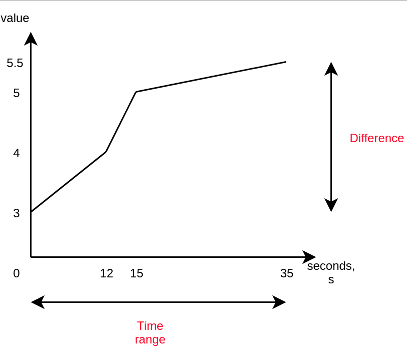
The nice thing about the rate() function is that it considers all data points, not just the first and last ones. Another function, irate, uses only the first and last data points.
You might now say… why not delta()? Well, rate() we have just described has this excellent characteristic: it automatically adjusts for resets. This means it is only suitable for constantly increasing metrics, a.k.a. the metric type called a “counter”. It’s not ideal for a “gauge”. Also, a keen reader would have noticed that using rate() is a hack to work around the limitation that floating-point numbers are used for metrics’ values and cannot go up indefinitely, so they are “rolled over” once a limit is reached. This logic prevents us from losing old data, so using rate() is a good idea when you need this feature.
Note: Because of this automatic adjustment for resets, if you want to use any other aggregation together with rate(), you must apply rate() first; otherwise, the counter resets will not be caught, and you will get weird results.
Either way, PromQL currently will not prevent you from using rate() with a gauge, so it is essential to realize which metric should be passed to this function when choosing. Using rate() with gauges is incorrect because the reset detection logic will mistakenly catch the values going down as a “counter reset”, and you will get wrong results.
All in all, let’s say you have a counter metric that is changing like this:
- 0
- 4
- 6
- 10
- 2
The reset between “10” and “2” would be caught by irate() and rate() and it would be taken as if the value after that were “12” i.e. it has increased by “2” (from zero). Let’s say that we were trying to calculate the rate with rate() over 60 seconds, and we got these six samples on ideal timestamps. So, the resulting average rate of increase per second would be:
12-0/60 = 0.2. Because everything is perfectly ideal in our situation, the opposite calculation is also true: 0.2 * 60 = 12. However, this opposite calculation is not always true when some samples do not cover the full range ideally or when samples do not line up perfectly due to random delays introduced between scrapes. Let me explain this in more detail in the following section.
Extrapolation: what rate() does when missing information
Last, it’s essential to understand that rate() performs extrapolation. Knowing this will save you from headaches in the long term. Sometimes, when rate() is executed at a point, some data might be missing if some scrapes fail. Moreover, the scrape interval due to added randomness might not align perfectly with the range vector, even if it is a multiple of the range vector’s time range.
In such a case, rate() calculates the rate with the data it has and then, if any information is missing, extrapolates the beginning or the end of the selected window using either the first or the last two data points. This means that you might get uneven results even if all of the data points are integers, so this function is suited only for spotting trends and spikes and for alerting if something happens.
Aggregation
Optionally, you apply rate() only to specific dimensions like other functions. For example, rate(foo) by (bar) will calculate the rate of change of foo for every bar (label’s name). This can be useful if you have, for example, haproxy running and you want to calculate the rate of change of the number of errors by different backends so you can write something like rate(haproxy_connection_errors_total[5m]) by (backend).
Examples
Alerting Rules
As described previously, rate() works perfectly when you want to get an alert when the number of errors jumps. So, you could write an alert like this:
groups:
- name: Errors
  rules:
  - alert: ErrorsCountIncreased
    expr: rate(haproxy_connection_errors_total[5m]) by (backend) > 0.5
    for: 10m
    labels:
      severity: page
    annotations:
      summary: High connection error count in {{ $labels.backend }}
This would inform you if any of the backends have increased connection errors. As you can see, rate() is perfect for this use case. Feel free to implement similar alerts for your services that you monitor with MetricFire. Interested in seeing what we can do for you? Try our free trial or sign up for a demo.
SLO Calculation
Another everyday use case for the rate() function is calculating SLIs and seeing if you do not violate your SLO/SLA. Google has recently released a popular book for site-reliability engineers. Here is how they calculate the availability of the services:
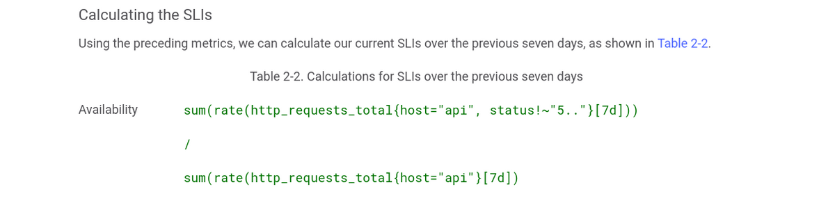
As you can see, they calculate the rate of change of the amount of all of the requests that were not 5xx and then divide by the rate of change of the total amount of requests. If there are any 5xx responses, the value would be less than one. You can, again, use this formula in your alerting rules with some specified threshold - then you would get an alert if it is violated, or you could predict the near future with predict_linear and avoid any SLA/SLO problems.
Practical Applications of rate()
1. Monitoring Request Rates:
To monitor the rate of incoming HTTP requests to a server:
promqlrate(http_requests_total[5m])
This provides the average number of requests per second over the last 5 minutes.
2. Alerting on High Error Rates:
To alert when the error rate exceeds a certain threshold:
promqlrate(http_errors_total[5m]) / rate(http_requests_total[5m]) > 0.05
This triggers an alert if more than 5% of requests result in errors over a 5-minute window.
3. Calculating Service Level Objectives (SLOs):
To assess whether a service meets its SLOs by calculating the success rate:
promql(rate(http_requests_total{status!~"5.."}[5m])) / rate(http_requests_total[5m])
This computes the proportion of successful requests (non-5xx status codes) over the total requests in the last 5 minutes.
Best Practices and Considerations
-
Use with Counters: The
rate()function is designed for use with counter metrics, which are expected to increase monotonically. Using it with non-counter metrics can yield misleading results.Medium+3Prometheus+3Prometheus+3 -
Avoiding Misinterpretation: Be cautious of interpreting short-term spikes or drops, especially with short time ranges, as they may not reflect actual trends.
-
Combining with Aggregation Functions: For a comprehensive view, combine
rate()with aggregation functions likesum()oravg()to analyze metrics across multiple instances or services.
What are other use cases for Prometheus functions?
There are as many Prometheus function use cases as there are functions—and even more. Below, we'll demonstrate just a few uses of Prometheus functions.
Aggregation operators
Aggregation operators calculate mathematical values over a time range. You can use Prometheus functions such as the ones below to aggregate over a given range vector:
- avg_over_time() for the average (mean) value
- max_over_time() for the maximum value
- count_over_time() for the total count of all values
Counting HTTP requests
As another example, you can use the increase() Prometheus function to count the number of HTTP requests over the past 5 minutes, e.g.:
increase(http_requests_total{job="api-server"}[5m])
Linear regression
Given a range vector and a scalar t, the predict_linear() Prometheus function uses simple linear regression to predict the future value of the time series t seconds.
Regular expressions
The label_replace() Prometheus function searches through time series to find one that matches the given regex (regular expression), and then.
Calculating percentiles
Given a histogram, the histogram_quantile() Prometheus function. The highest bucket in the histogram must have an upper bound of +Inf (positive infinity).
Calculating differences
Given a range vector, the delta() Prometheus function calculates the difference between two quantities. For example, to calculate the difference in CPU temperature between now and 2 hours ago:
delta(cpu_temp_celsius{host="zeus"}[2h])
To enhance your use of Prometheus functions, you can also integrate Prometheus with Grafana, a web application for data analytics and visualization. MetricFire's hosted Grafana service makes it easy for any Prometheus user to enjoy high-quality, informative data visualizations. When you choose MetricFire, you also get access to our Hosted Graphite data source and platform and 24/7 support for all your Graphite and Grafana needs. Sign up today!
How MetricFire Can Help
MetricFire is a cloud infrastructure and application monitoring platform that makes understanding your data at a glance simple. We offer a Hosted Graphite service that handles issues such as scaling, data storage, and support and maintenance—so that you can spend more time on the metrics and less on the technical details.
Conclusion
The rate() function is a powerful feature in Prometheus for analyzing the behavior of counter metrics over time. By understanding its operation and applying it appropriately, users can gain valuable insights into system performance, detect anomalies, and ensure that services meet their performance objectives.
To learn more, check out the Prometheus posts on our blog or book a demo to discuss your business needs and objectives. Want to get started with your monitoring right away? The MetricFire free trial is an excellent way to explore what you can do with hosted Graphite.

